While reading articles on Quarterly Review of Economics and Finance via Science Direct, I often find myself wondering how to get information of all stocks and indexes around the world right now to quickly reference against the article?
A very common stock database that I can basically look for any listed company on different stock markets is Yahoo! Finance.
By typing the company name or symbol on the search bar:

At best, I have the option to select the time frame I want to see for that stock, and then download the data. At worse, I have zero interested in downloading, manually, one stock by another! 🤦♀️
Some examples: 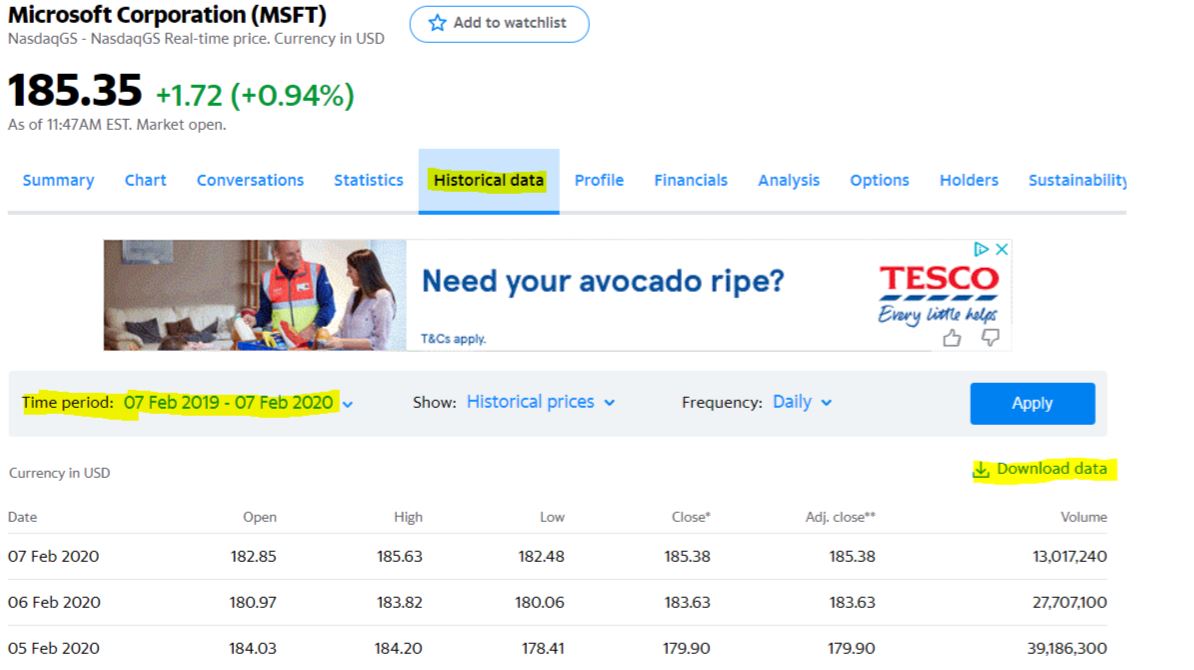
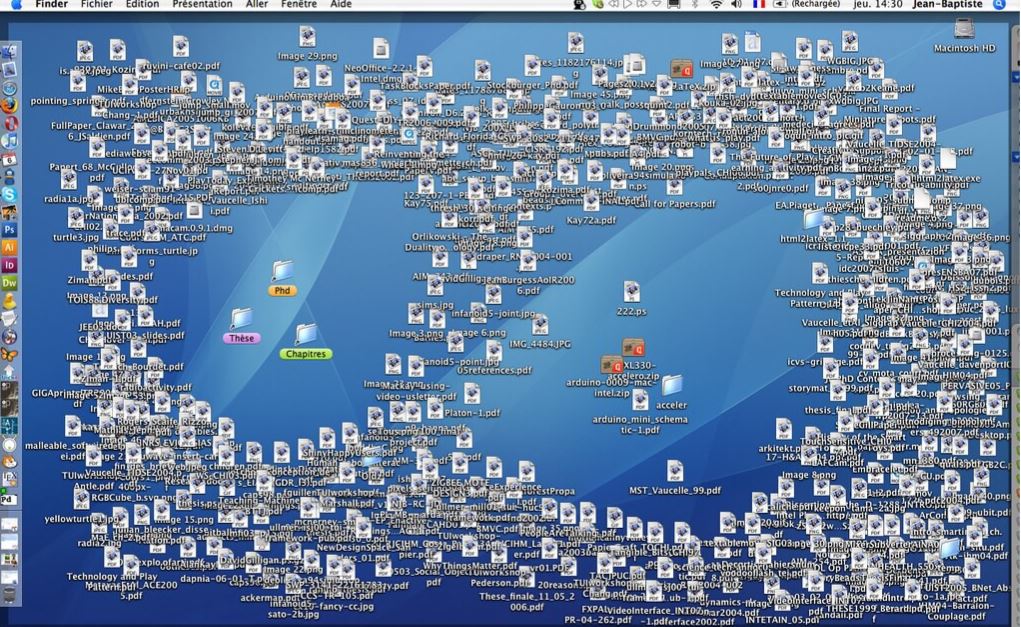
And my personal favourite example:
So last week, while waiting for my housemate to decide what to eat for dinner, I looked up on the internet and found out that these stock data can be directly accessed from our python notebook!
What is cool about this? You can get data from any share you want, selecting the dates you wish to analyse, all that without downloading NOTHING AT ALL! I don’t know you, but I love when I don’t need to add another file to my already messy computer.
So I just developed my own script to query any stocks and perform some basic financial analysis on these data. Below are some more details you could expect:
- I query stocks data from Yahoo Finance, with given date range and stock list. Then, I visualise their closing prices as well as daily return.
- I query ALL stock indexes from Yahoo Finance, with given date range. Then I visualise daily return for equally weighted market portfolio
The script is simple.
Part A: Individual Stocks
First we will need to install and load the libraries need, including pandas_datareader – information to be retrieved with the supports of that library;
# Typical libraries for data manipulation and visualisation
import pandas
import datetime
import numpy
import matplotlib.pyplot as plt
from matplotlib import style
import plotly.express as px
import warnings
warnings.filterwarnings("ignore")

# For reading stock data from yahoo
import pandas_datareader as web
import yfinance as yf

# For time stamps
from datetime import datetime
For a customised stock portfolio, we will store the stock symbol into a data frame
# The tech stocks we'll use for this analysis
tech_list = ['AAPL','GOOG','FB','AMZN']
And define the date range for the data
end = datetime.now() #or end = datetime(2021,2,20)
start = datetime(2017,1,3)
Get the data using datareader library and then display the first rows of the dataframe to see what they look like
prices = web.DataReader(tech_list, 'yahoo', start, end)['Adj Close']
prices.head()
Quick glance into their daily closing prices movement with plotly visualisation
#viz
import plotly.graph_objects as go
from plotly.subplots import make_subplots

fig = make_subplots(rows=2, cols=2, start_cell="bottom-left",
                   subplot_titles=("APPLE", "GOOGLE", "Facebook", "Amazon"))

fig.add_trace(go.Scatter(x=prices.index, y=prices['AAPL'], name = 'Apple'),
              row=1, col=1)

fig.add_trace(go.Scatter(x=prices.index, y=prices['GOOG'], name = 'Google'),
              row=1, col=2)

fig.add_trace(go.Scatter(x=prices.index, y=prices['FB'], name = 'Facebook'),
              row=2, col=1)

fig.add_trace(go.Scatter(x=prices.index, y=prices['AMZN'], name = 'Amazon'),
              row=2, col=2)

fig.update_layout(
    width = 900,
    height = 700,
    title = "Daily closing Prices of FAAG stock group")

fig.show()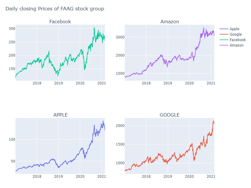
And we also want to analyse the return of the stock.
# We'll use pct_change to find the percent change for each day
returns =prices.pct_change()
returns.head()
Part B: All stock indices around the world
We will first retrive a list of major Stock Indices around the world, then run a loop to collect historical data of these All stock indices.
#list of Stock Indices
df_list = pandas.read_html('https://finance.yahoo.com/world-indices/')
majorStockIdx = df_list[0]
#collect historical data
stock_list = []
for s in majorStockIdx.Symbol: # iterate for every stock indices
    # Retrieve data from Yahoo! Finance
    tickerData = yf.Ticker(s)
    tickerDf1 = tickerData.history(period='1d', start='2010-01-01', end='2020-10-30')
    # Save historical data
    tickerDf1['ticker'] = s # don't forget to specify the index
    stock_list.append(tickerDf1)
    # Concatenate all data
    msi = pandas.concat(stock_list, axis = 0)
Now to clasify each of the indices to its region, we can define a function:
def getRegion(ticker):
    for k in region_idx.keys():
        if ticker in region_idx[k]:
            return k
where
region_idx= { 'US & Canada' : ['^GSPC', '^DJI', '^IXIC', '^RUT','^GSPTSE'],
               'Latin America' : ['^BVSP', '^MXX', '^IPSA', ],
               'East Asia' : ['^N225', '^HSI', '000001.SS', '399001.SZ', '^TWII', '^KS11'],
               'ASEAN & Oceania' : ['^STI', '^JKSE', '^KLSE','^AXJO'],
               'South & West Asia' : ['^BSESN', '^TA125.TA'],
               'Europe' : ['^FTSE', '^GDAXI', '^FCHI', '^STOXX50E','^N100', '^BFX']
              }
Create a new column to store the region information in our stock indices data frame
msi['region']= msi.ticker.apply(lambda x: getRegion(x))
lastDate = msi.loc[msi.Date == '2020-09-30'].reset_index().drop(['index'],axis=1)
lastDate.head()
cols = ['Date', 'ticker', 'region', 'Open', 'High', 'Low', 'Close', 'Volume', 'Dividends',
       'Stock Splits', 'Adj Close']
lastDate = lastDate[cols]
def nearest(dates, dateRef):

    dts = pandas.to_datetime(dates)
    drf = pandas.to_datetime(dateRef)

    prevDate = dts[dts < drf]
    return prevDate[-1]

def getReturn(period, number, ticker, dt, val):

    df = msi.loc[msi.ticker == ticker].reset_index()
    existingDates = df['Date'].unique()

    if period == 'Y':
        dtp = (pandas.Timestamp(dt) - pandas.DateOffset(years=number))
    elif period == 'M':
        dtp = (pandas.Timestamp(dt) - pandas.DateOffset(months=number))
    elif period == 'W':
        dtp = (pandas.Timestamp(dt) - pandas.DateOffset(weeks=number))
    elif period == 'D':
        dtp = (pandas.Timestamp(dt) - pandas.DateOffset(days=number))

    df['Date_pd'] = pandas.to_datetime(df['Date'])
    if dtp in existingDates:
        return (val/df.loc[df.Date_pd == dtp, "Close"].values[0] - 1)*100
    else:
        closestDate = nearest(existingDates, dtp)
        return(val/df.loc[df.Date_pd == closestDate, "Close"].values[0] - 1)*100

lastDate['1DR'] = lastDate.apply(lambda r: getReturn('D', 1, r.ticker, r.Date, r.Close), axis =1)
lastDate['1WR'] = lastDate.apply(lambda r: getReturn('W', 1, r.ticker, r.Date, r.Close), axis =1)
lastDate['1MR'] = lastDate.apply(lambda r: getReturn('M', 1, r.ticker, r.Date, r.Close), axis =1)
lastDate['3MR'] = lastDate.apply(lambda r: getReturn('M', 3, r.ticker, r.Date, r.Close), axis =1)
lastDate['6MR'] = lastDate.apply(lambda r: getReturn('M', 6, r.ticker, r.Date, r.Close), axis =1)
lastDate['1YR'] = lastDate.apply(lambda r: getReturn('Y', 1, r.ticker, r.Date, r.Close), axis =1)
lastDate['3YR'] = lastDate.apply(lambda r: getReturn('Y', 3, r.ticker, r.Date, r.Close), axis =1)
Then plotting returns for these Stock Indices would be easy:
palette = ["#965757", "#D67469", "#4E5A44", "#A1B482", '#EFE482', "#99BFCF"]
fig, axes = plt.subplots(1,5, figsize=(20, 10),sharey=True)
width = 0.75
cols = ['1MR', '3MR', '6MR','1YR','3YR']
for i, j in enumerate(cols):
    ax = axes[i]
    tick = lastDate.ticker.apply(lambda t : ticker[t])
    ax.barh(tick,lastDate[j], width, color = palette[i])
    ax.set_title(j, fontweight ="bold")
    ax.invert_yaxis()

fig.text(0.5,0, "Return (%)", ha="center", va="center", fontweight ="bold")
fig.text(0,0.5, "Stock Indices", ha="center", va="center", rotation=90, fontweight ="bold")
fig.suptitle("Returns for Major Stock Indices based on 30 September 2020", fontweight ="bold",y=1.03, fontsize=14)
fig.tight_layout()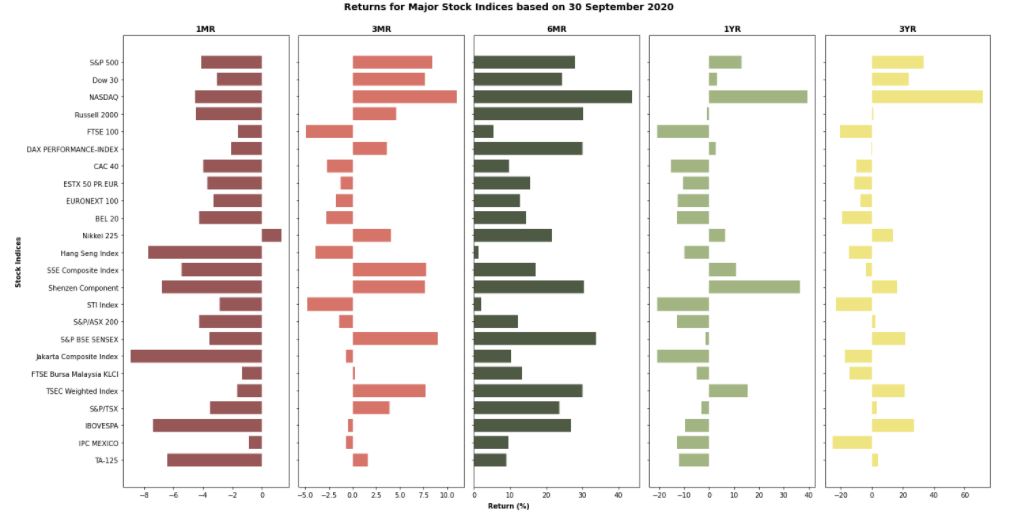
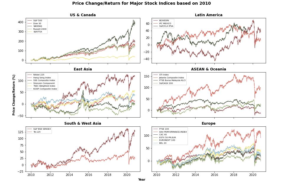
Similar methodology, we can also produce this chart quickly:
You can find my notebook code here (https://github.com/Rachelios/A-cup-of-tea-and-a-good-book/tree/master/Stock%20Markets)